Hands-on machine learning met Python

Lecture 3 - Introduction to Big Data for Lean

Vandaag

Werkwijze

• Python als rekenwerktuig
• AI als sparringpartner
• Testsets als laatste controle

Vier mini-projecten

• Lineaire regressie
• Neurale netwerken
• Beslissingsbomen
• Bayesiaanse onzekerheid

Zie ugain.naert.net voor meer uitleg!

1 . Werkomgeving en AI

Drie routes naar Python

JupyterLite

Geen installatie.

Goed voor snel starten, maar beperkt in packages en rekenkracht.

Google Colab

Cloud-notebooks.

Handig voor TensorFlow, maar afhankelijk van account, netwerk en sessies.

Lokaal met VS Code

Aanbevolen op lange termijn.

Gebruik Python 3.12 of 3.13; Python 3.14 is voorlopig minder geschikt voor TensorFlow.

Tip

Als je zelf Python ervaring hebt: gebruik eigen, lokale omgeving met uv (of conda). Zo niet: kies liefst voor Colab met Jupyter Lite als backup.

AI gebruiken zonder stuurloos te worden

AI helpt

• plan voorstellen
• code schrijven
• foutmeldingen uitleggen
• alternatieven vergelijken

Jij beslist

• wat de vraag is
• welke fout belangrijk is
• of er datalek is
• wat de conclusie mag zijn

Tip

Vraag eerst om een plan. Laat daarna stap per stap code maken en uitvoeren.

Welke AI-assistent?

Online taalmodellen

• ChatGPT
• Claude
• Gemini

Werken via de browser en zijn genoeg om met de startprompts uit deze les te werken.

Code-assistenten

• GitHub Copilot
• Claude Code
• Cursor

Handig in een editor of terminal, vooral als je vaker programmeert.

Tip

Voor deze les volstaat een online taalmodel. Gebruik het als sparringpartner: lees het plan, voer code in kleine stappen uit en blijf zelf controleren.

2 . Lineaire regressie

Vraag

Wanneer wordt een flexibeler model beter, en wanneer begint het ruis te leren?

Dataset: California Housing.
Taak: voorspel mediane huiswaarde uit mediaan inkomen.

Dataset en concept

California Housing

• 20.640 geografische blokgroepen
• doelvariabele: MedHouseVal
• input in deze oefening: MedInc

Modelcomplexiteit

• graad 1: rechte lijn
• hogere graad: flexibeler
• validatiefout kiest de graad
• testset blijft buiten beeld

Wat de AI moet doen

Goed

• testset eerst apart zetten
• 5-voudige cross-validatie
• preprocessing in een Pipeline
• training en validatie vergelijken

Niet goed

• testset gebruiken om de graad te kiezen
• schaling buiten de folds leren
• een perfecte U-vorm beloven
• alleen de trainingsfout tonen

Resultaat: polynomiale regressie

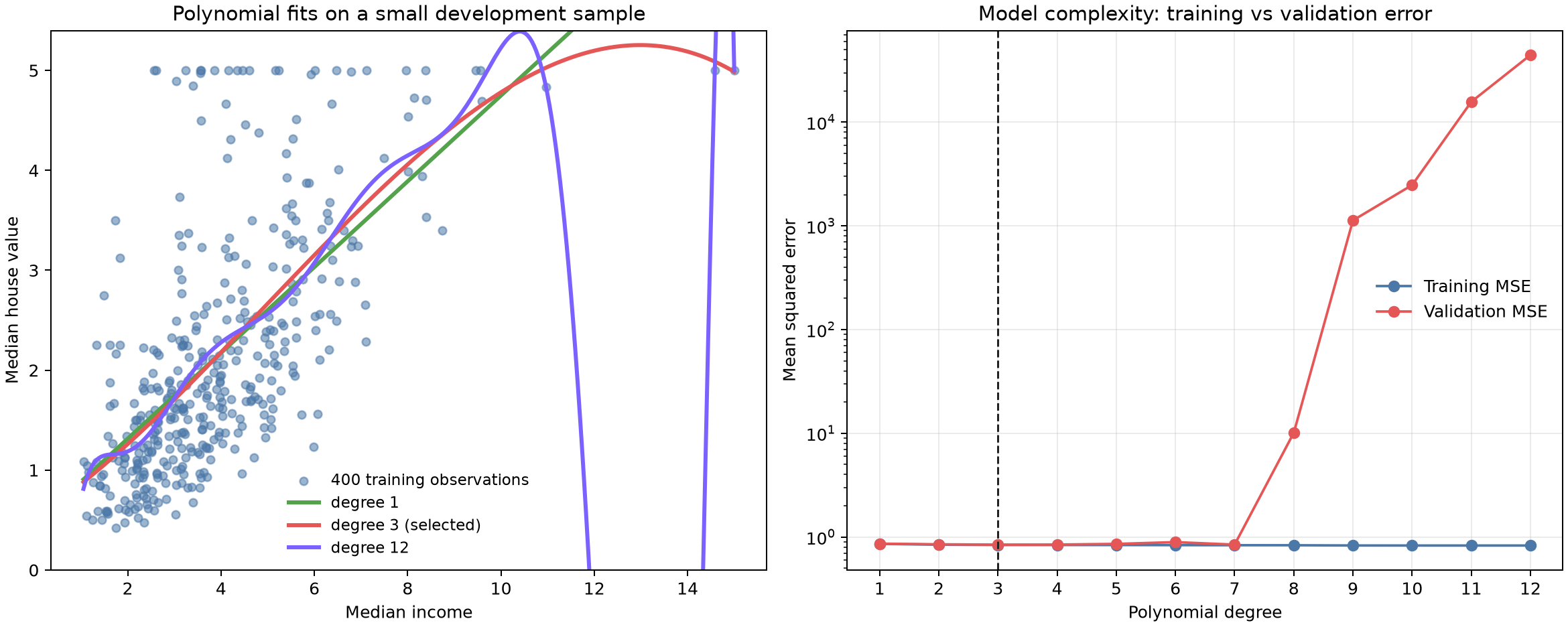
Wat valt op?

Signaal

Graad 1 is stabiel, maar beperkt.

Een kleine extra kromming helpt.

Waarschuwing

Hoge graden kunnen numeriek en statistisch instabiel worden.

De validatiefout verraadt dat. De trainingsfout niet.

Note

De y-as van de foutgrafiek is logaritmisch omdat de slechtste graden zo hard ontsporen.

Startprompt

Use scikit-learn and the California Housing dataset to investigate model
complexity in polynomial regression. Predict MedHouseVal from MedInc. Reserve
20% of the complete dataset as an untouched test set, then draw a reproducible
sample of 400 observations from the remaining development data.

Compare polynomial degrees 1 through 12 using five-fold cross-validation. Keep
all scaling and polynomial transformations inside a Pipeline. Use training and
validation MSE to select the degree; do not inspect the test set.

Make the fitted curves and training-versus-validation error curve understandable.
After selecting the degree, fit the final model on the 400 development
observations and use the test set once to report MSE and R2. First propose a
short plan. Do not write code yet.

3 . Neurale netwerken

Vraag

Hoe zie je dat een groot netwerk blijft leren op training, maar niet meer op nieuwe data?

Dataset: Fashion-MNIST.
Taak: classificeer kleine afbeeldingen van kledingstukken.

Dataset en concept

Fashion-MNIST

• 70.000 grijswaardenbeelden
• 10 kledingcategorieen
• 60.000 ontwikkeling, 10.000 test

Leren doorheen de tijd

• trainingsverlies volgt de updates
• validatieverlies meet generalisatie
• een groeiende kloof wijst op overfitting

Leercurven

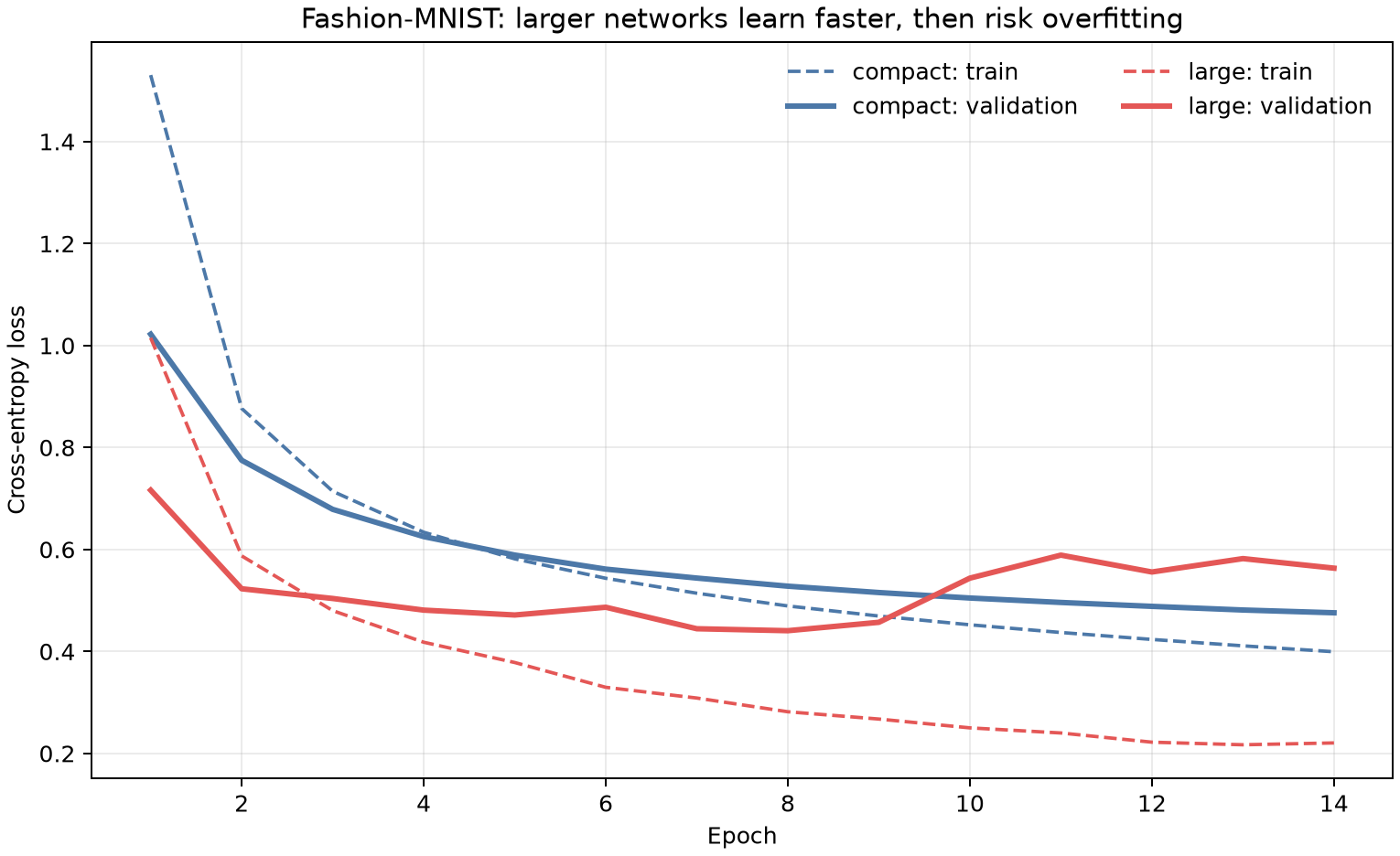
De les

Compact model

Langzamer, maar stabiel.

Validatieverlies blijft rustig dalen.

Groter model

Leert sneller.

Na enkele epochs daalt training verder terwijl validatie slechter wordt.

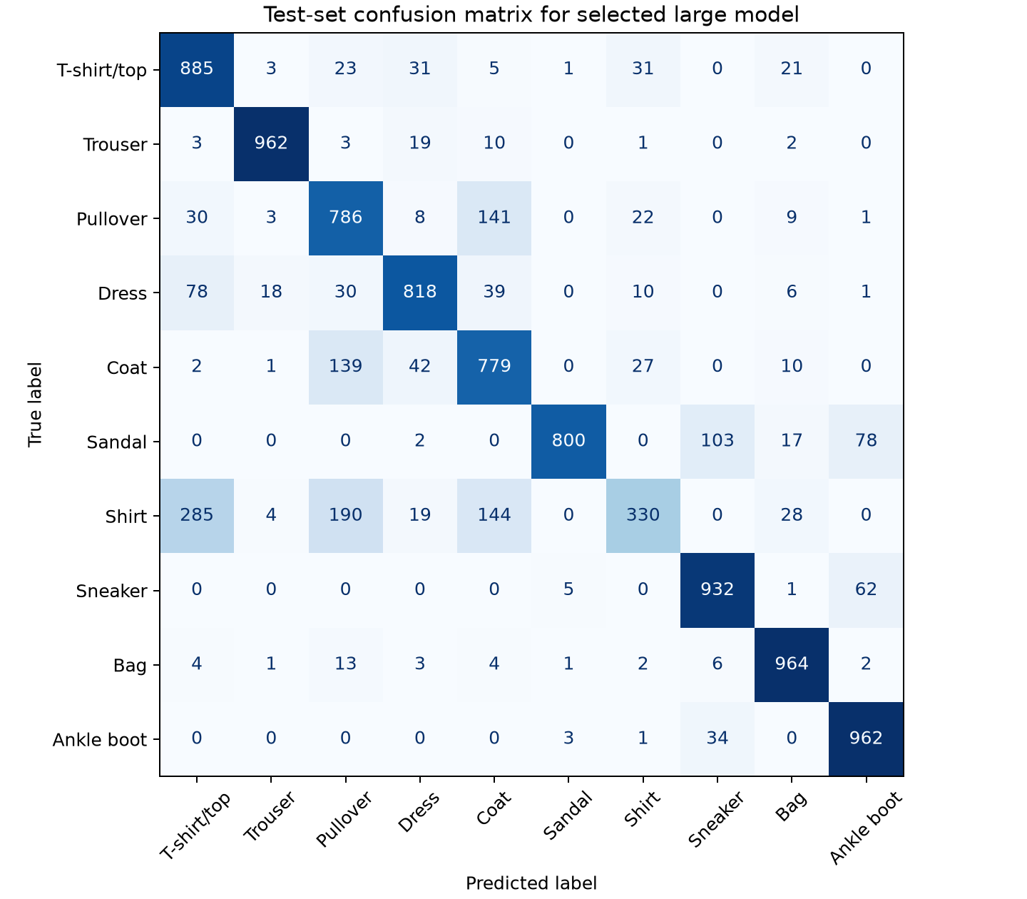
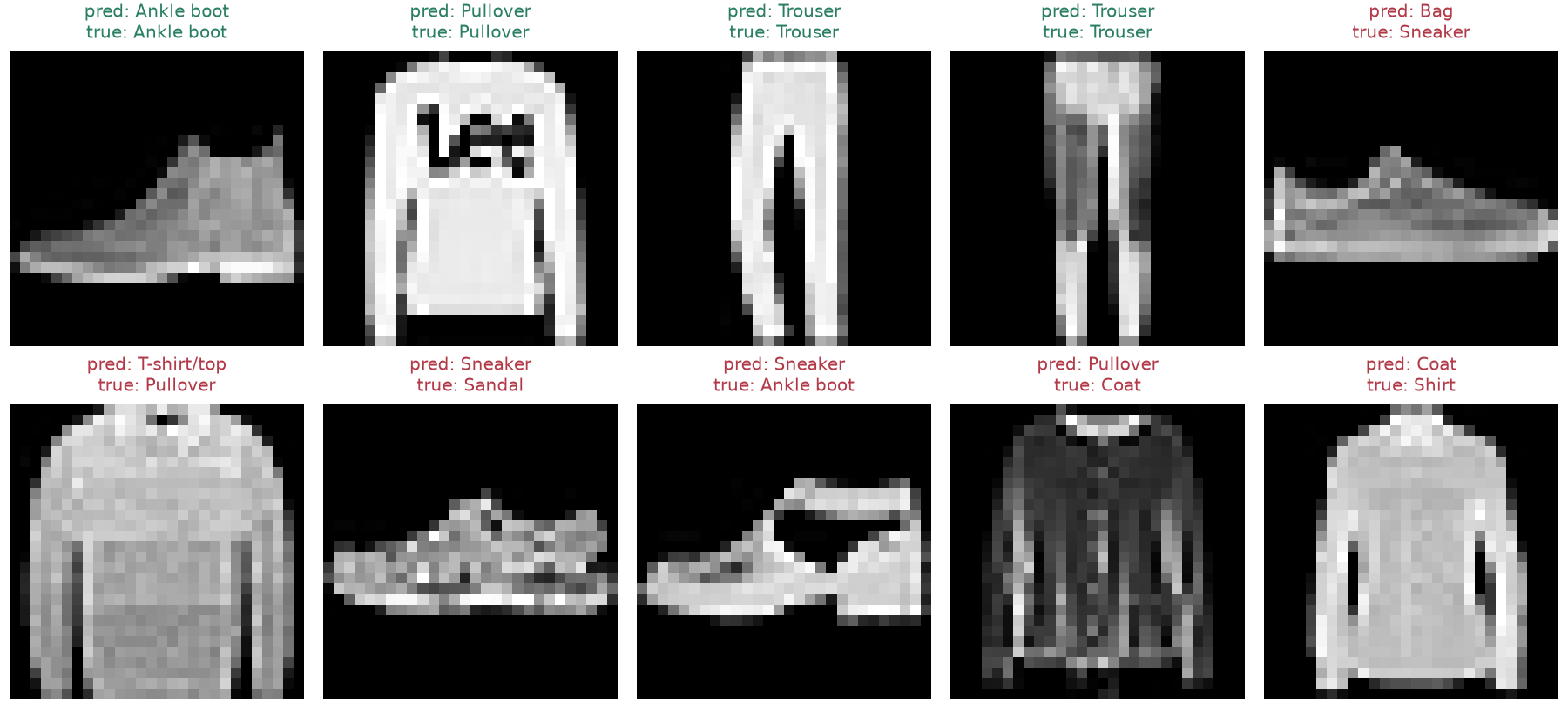
Waar maakt het model fouten?

Denkvragen

• Welke klassen lijken visueel op elkaar?
• Is accuracy genoeg, of wil je per klasse kijken?
• Wat zou een CNN beter benutten dan een dense netwerk?
• Waar zou early stopping het model gekozen hebben?

Startprompt

Use Keras to compare a compact dense neural network with a substantially larger
one on Fashion-MNIST. The goal is to investigate how model capacity affects
training and validation loss and when overfitting becomes visible.

Use a limited, reproducible and stratified sample from the official development
data so the exercise remains quick. Keep the official test set completely
separate until all choices have been made. Choose and motivate suitable
architectures, preprocessing, loss function, optimizer and number of epochs.

Visualize training and validation loss per epoch for both models. Then evaluate
only the selected model once on the test set. Show predictions and a confusion
matrix. Do not claim overfitting unless the learning curves provide evidence.

4 . Beslissingsbomen op Titanic

Vraag

Wat win je en verlies je wanneer je van een kleine boom naar een forest gaat?

Dataset: Titanic.
Taak: voorspel overleving uit klasse, geslacht, leeftijd, familie en tarief.

Dataset en concept

Titanic

• 891 passagiers
• doelvariabele: survived
• ontbrekende waarden in age

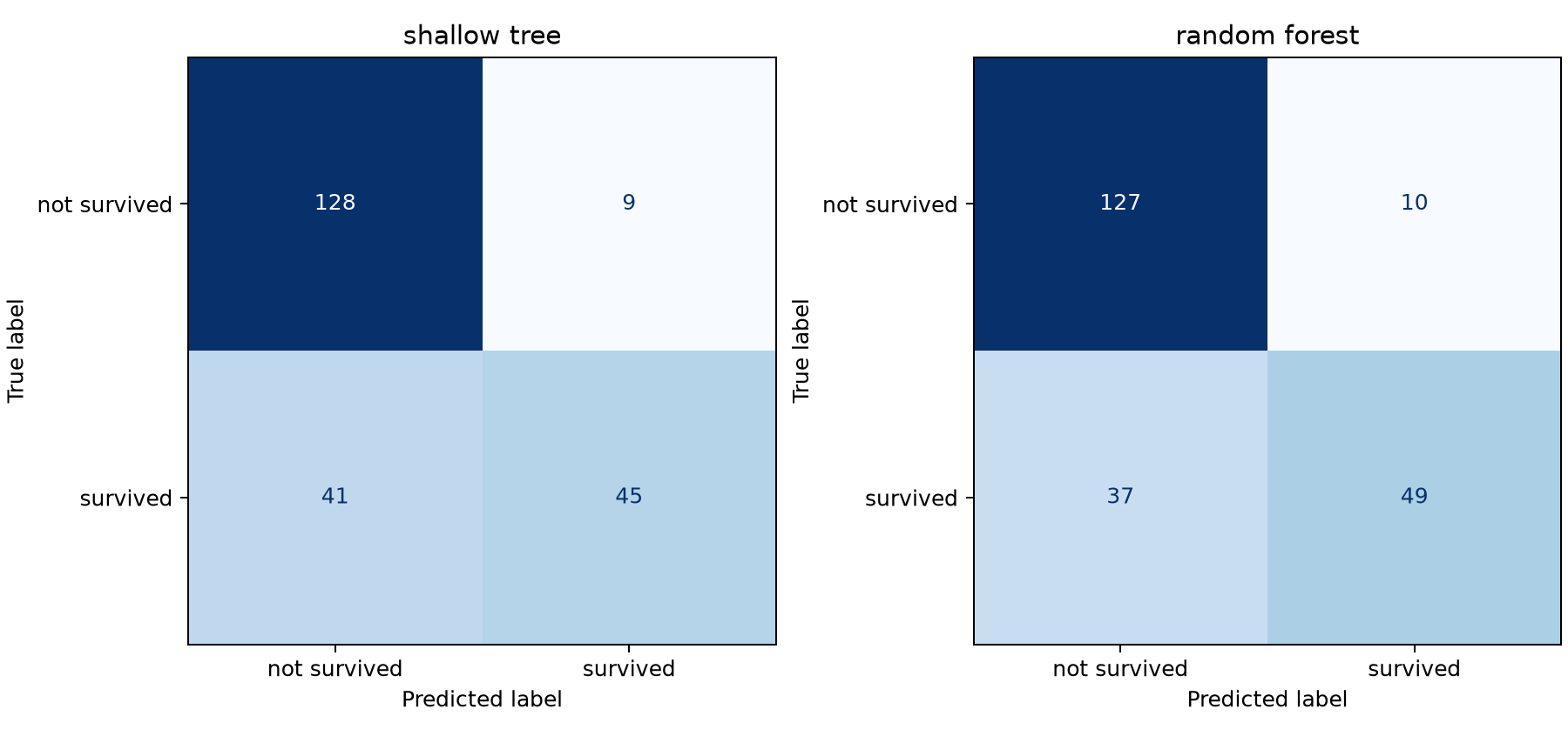
Confusion matrix

• positief = overleefd
• precision: voorspelde overlevenden
• recall: werkelijke overlevenden gevonden

Discipline: train, validatie, test

Train

Leer imputatie, encoding en modelparameters.

Validatie

Vergelijk boom en forest via cross-validatie binnen de trainingdata.

Test

Een keer gebruiken nadat de instellingen gekozen zijn.

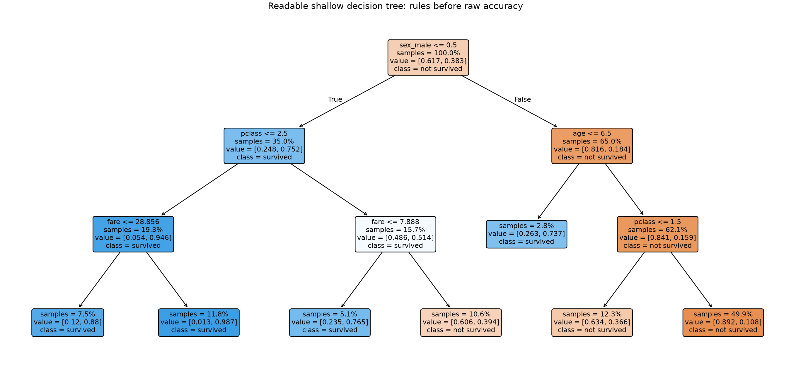
Interpreteerbare boom

Confusion matrices

Interpretatie

Boom

Direct uitlegbaar.

Maar een kleine boom mist veel werkelijke overlevenden.

Forest

Iets betere recall voor overleven.

Maar geen enkele boom vat het hele model samen.

Startprompt

Write Python code that trains a decision tree and a random forest on the Titanic
dataset to predict passenger survival. Use pclass, sex, age, sibsp, parch and
fare.

Start with a stratified train/test split and keep the test set untouched until
the final evaluation. On the training data only, use cross-validation to compare
a shallow decision tree with a random forest and, if needed, tune hyperparameters.

Impute missing numerical values using medians learned exclusively inside each
training fold, and encode categorical features inside the same workflow. Prefer
a scikit-learn Pipeline. Do not remove observations merely because age is
missing.

After choosing settings, fit both models on the full training data. Only then
evaluate them once on the test set. Report accuracy, precision, recall and F1
for the survived class; show test-set confusion matrices and a readable tree.

5 . Bayesiaanse onzekerheid

Vraag

Kunnen we niet alleen het gemiddelde voorspellen, maar ook de onzekerheid laten meegroeien?

Dataset: restaurantfooien.
Taak: voorspel fooi uit het totale bedrag.

Dataset en concept

Tips

• 244 restaurantbetalingen
• input: total_bill
• doel: tip

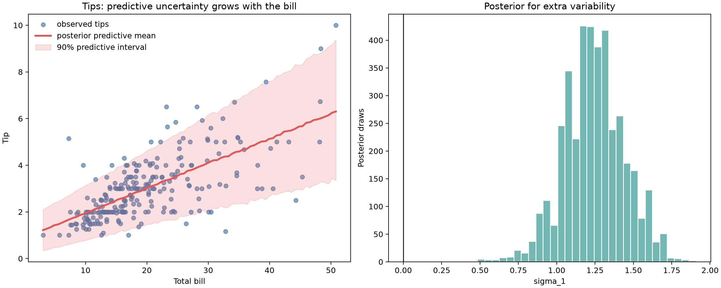
Heteroscedasticiteit

De spreiding kan toenemen naarmate de rekening hoger wordt.

We modelleren dus gemiddelde en standaardafwijking.

Model

\[ y \sim \mathcal{N}(\mu(x), \sigma(x)) \]

\[ \mu(x) = \alpha + \beta x,\qquad \sigma(x) = \sigma_0 + \sigma_1 x \]

Note

Omdat \(\sigma_1 \geq 0\) nemen we vooraf aan dat de spreiding gelijk blijft of stijgt.

Posterior predictive

MCMC in de praktijk

Modelcontrole

• geen onnodige latente variabelen
• vectorized likelihood
• geschaalde input
• posterior predictive uit draws

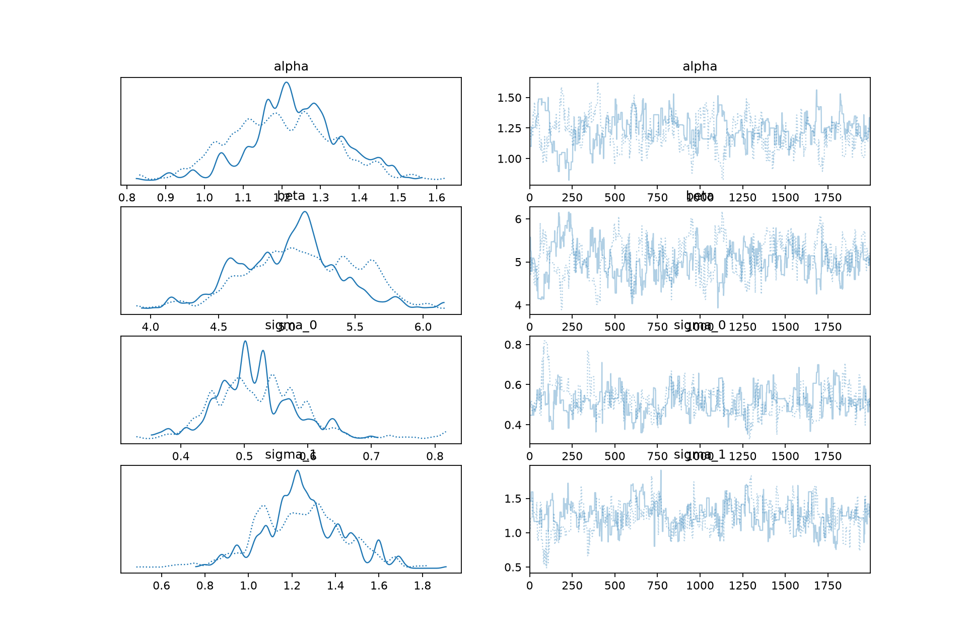
Rekencontrole

• meerdere MCMC-ketens
• R-hat en ESS bekijken
• divergences controleren
• traceplots inspecteren

Traceplots

Startprompt

Use PyMC to fit a heteroscedastic Bayesian regression model to the seaborn Tips
dataset. Predict tip from total_bill and rescale total_bill to [0, 1].

    tip ~ Normal(mu(x), sigma(x))
    mu(x)    = alpha + beta * x_scaled
    sigma(x) = sigma_0 + sigma_1 * x_scaled

Use sensible normal priors for alpha and beta and half-normal priors for sigma_0
and sigma_1. Use prior-predictive simulation before fitting the model.

Sample the posterior using MCMC. Summarize and interpret all four parameters,
and check convergence using R-hat, effective sample size, trace plots and the
number of divergences. Explain what sigma_1 says about changing variability,
while recognizing that the half-normal prior assumes variability cannot decrease.

Use posterior-predictive draws to visualize the fitted relationship and its
uncertainty. Do not construct a posterior-predictive interval merely by plugging
posterior mean parameters into mu +/- sigma.

Studiewijzer

Niet te kennen voor het examen